Four experiments, one model, one question: what does stability actually look like in a small language model, and what breaks it?
The model is GPT-2 Small — 12 transformer layers, 12 attention heads, 768-dimensional embeddings, 85.7M parameters. Trained on FineWeb-Edu, a filtered educational subset of Common Crawl. Each run records 8 signals throughout training. Before diving in, here is what those signals mean:
- Loss (train / val) — cross-entropy over the next-token prediction task. Lower is better. A model initialized at random over a 50,257-token vocabulary starts at ln(50,257) ≈ 10.82 by definition. As it learns, this drops.
- Gradient norm — the total magnitude of the gradient vector computed at each step, before any clipping. A health indicator: a well-behaved run has a gradient norm that is high early, then settles. Persistent spikes or erratic behavior signal unstable optimization.
- Parameter norm — the total L2 magnitude of all model weights combined. Grows steadily throughout training as weights move away from their initialized values. Large sudden swings indicate instability.
- Update-to-weight ratio — how large each weight update is relative to the weight’s current magnitude. The conventional healthy range is around 1e-3 (0.1%). Much lower and the optimizer has effectively stalled; much higher and updates are oversized relative to what the weights can absorb.
- Activation statistics (mean, std) — the distribution of values flowing through the network’s final layer. A healthy run keeps the mean near zero and the standard deviation in a stable range throughout training.
Exp 01 — Baseline
What this experiment asks: before testing what breaks, we need to know what healthy looks like. This run trains GPT-2 Small to completion with standard settings — no modifications. Every subsequent experiment is compared against it.
Config. 1 billion tokens, 1907 optimizer steps. The effective batch size is 524,288 tokens per step — computed as 8 samples × 64 gradient accumulation steps × 1024 token context window. Gradient accumulation means running 64 small forward passes before doing a single weight update, which simulates a much larger batch without requiring proportionally more GPU memory.
Optimizer: AdamW (explained in Exp 02). Learning rate: cosine schedule from 6e-4 down to 6e-5 over the full run, with a 50-step warmup (explained in Exp 02). Gradient clipping at 1.0. Precision: BF16 — a 16-bit floating point format that keeps the same numerical range as 32-bit, so there is no risk of overflow. On Blackwell tensor cores this gives a 2.4× throughput improvement over full precision (13k → 30.5k tokens/sec).
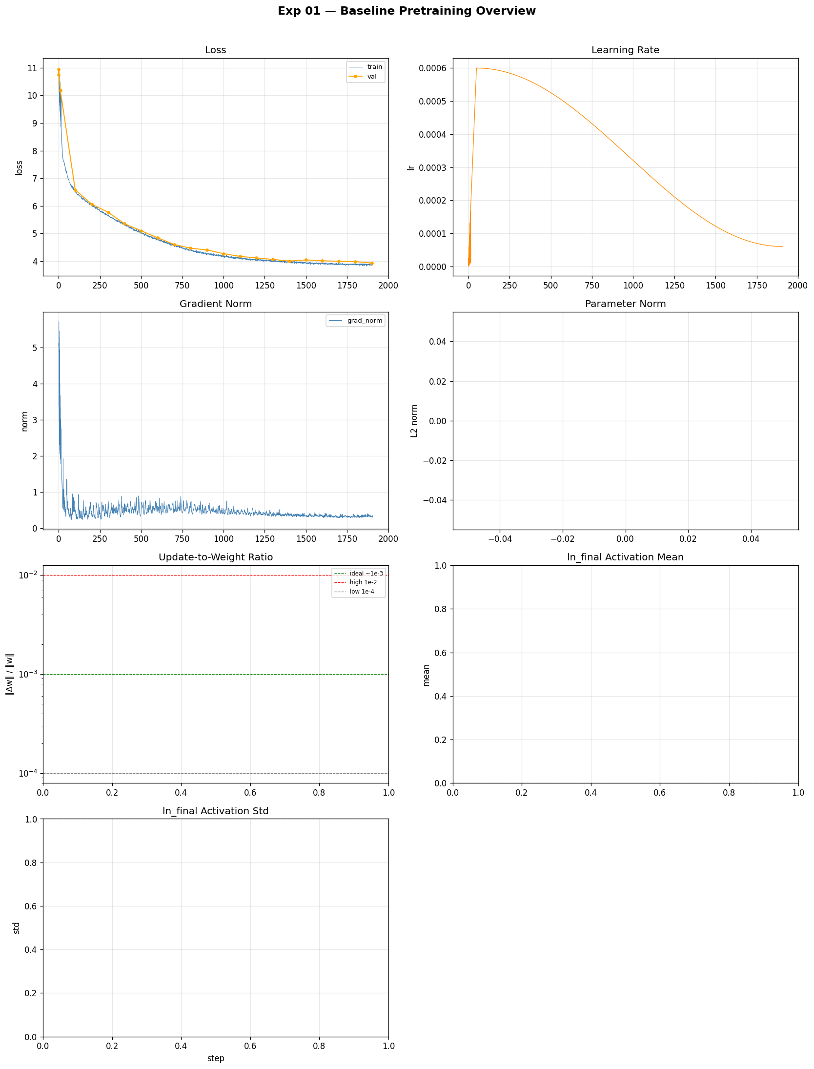
8 metrics across 1907 steps. The baseline everything else is compared against.
Loss started at 10.82 — exactly where random initialization lands — and dropped to around 4 by end of training. Train and val loss tracked closely throughout: you cannot meaningfully overfit a 124M parameter model on 1B tokens from a large varied corpus. The final ~4 is the reference point for all variants.
Gradient norm showed spikes during the warmup phase. This is expected: random initialization places the model in a high-curvature region of the loss landscape — a zone where the surface bends sharply, so gradients are large in magnitude and point in inconsistent directions across different training batches. Warmup ramps the learning rate from near-zero, keeping step sizes small while these large incoherent gradients exist. Once warmup ends and the model has moved to a smoother region, the norm settles.
Parameter norm climbed slowly and steadily — the model’s weights are growing away from their initialized values, which is normal. Update-to-weight ratio sat near the target 1e-3 at peak learning rate, drifting down gradually as the cosine schedule reduced the LR. Activations at the final layer stayed near zero mean with stable standard deviation throughout. Nothing unusual — this is what a healthy run looks like.
Exp 02 — Optimizer × Warmup
What this experiment asks: two of the most fundamental training decisions are the choice of optimizer and whether to use a learning rate warmup. Each is tested as a binary switch. The question is which one actually drives the outcome — and whether the two interact.
Adam and AdamW. Both are adaptive gradient optimizers: instead of applying the same learning rate to every weight, they maintain per-parameter estimates of past gradient magnitudes and use these to scale each weight’s step size individually — parameters with consistently large gradients get a smaller effective learning rate, and vice versa. The difference between Adam and AdamW is how weight decay is handled.
Weight decay is a regularization technique that gradually shrinks each weight toward zero at every step, preventing any single weight from growing unchecked. In vanilla Adam, weight decay is implemented as an L2 gradient penalty, which means it gets scaled by the same adaptive factor as the gradient — so heavily-updated parameters get proportionally less decay. AdamW decouples weight decay from the gradient update: it applies a fixed proportional shrink to each weight directly, independent of gradient history. This makes regularization cleaner and more predictable.
Warmup. At the very start of training, Adam’s second moment estimate v_t — its running average of squared gradients per parameter — is initialized at zero. The effective step size for each parameter is lr / sqrt(v_t), which becomes enormous when v_t is near zero. This is the cold-start problem: before the optimizer has seen enough gradients to build reliable estimates, its adaptive scaling misfires and step sizes are huge. Warmup addresses this by ramping the learning rate from near-zero to its target over the first N steps, keeping actual updates small while v_t stabilizes. With β2=0.95 — the decay rate for the second moment — the effective memory is roughly 20 steps, so a 50-step warmup is precisely calibrated to let v_t converge before full LR is applied.
| Variant | Optimizer | Warmup steps |
|---|---|---|
| A | Adam | 0 (no warmup) |
| B | Adam | 50 |
| C | AdamW | 0 (no warmup) |
| D | AdamW | 50 ← baseline |
All other settings identical to Exp 01. 1907 steps each.
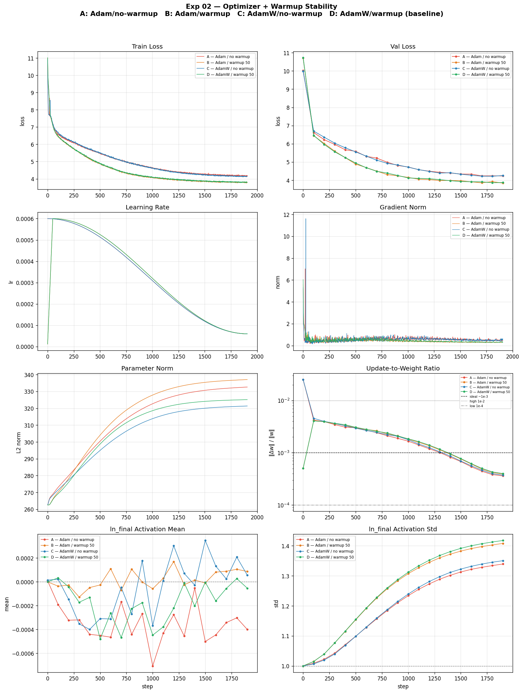
4 variants overlaid. Warmup is the dominant axis. Optimizer choice is secondary at this scale.
The warmup result is unambiguous. Variants A and C — no warmup, different optimizers — track together at a higher loss throughout the entire run. The gap opens in the first 50 steps and never closes. This is the cold-start problem playing out exactly as predicted: without warmup, enormous effective step sizes in the first ~20 steps push the model into a worse region of the loss landscape before the optimizer has reliable curvature estimates, and the model never fully recovers.
The optimizer result is more subtle. Adam vs AdamW produces no distinguishable difference in loss curves. The separation appears only in gradient norm, and only after ~750 steps — AdamW shows noticeably better damping of fluctuations. The timing is meaningful: weight decay needs ~750 steps to accumulate enough regularization pressure to visibly constrain parameter growth. Early in training the decay term is small relative to the gradient signal. It is a slow-burn effect, invisible to the loss curve on a data-rich corpus, visible only in gradient stability over the long run.
One anomaly worth flagging. The no-warmup variants end with smaller parameter norms than their warmup counterparts — counterintuitive, since no-warmup applied larger steps early. This does not have a clean explanation from the current data and is worth revisiting with per-layer norm tracking.
Activation mean drift. Variant C — AdamW without warmup — shows the mean of the final-layer activations drifting upward after ~1000 steps while all other variants stay near zero. The combination matters: without warmup, the first ~20 steps push weight matrices into asymmetric configurations before the optimizer has reliable estimates. Decoupled weight decay then shrinks all weights proportionally — but if certain directions were pushed systematically positive by those early noisy steps, decay shrinks them more slowly than new gradient signal pushes them further. Adam without warmup (variant A) does not trigger the same mechanism because there is no decoupled weight decay to reinforce the asymmetry.
The magnitude is small at 12 layers. The concern is the trend — in a deeper or longer run, this kind of drift shifts the effective operating point of every layer normalization downstream.
Takeaway: warmup is load-bearing. Optimizer choice is secondary at this scale and data regime.
Exp 03 — Initialization × Depth
What this experiment asks: once the optimizer is settled, the question moves to initialization — the values assigned to model weights at the start of training, before any data is seen. A deeper model has more layers, and each layer writes its output back into a shared running vector called the residual stream. If every layer adds signal with the same random scale, the variance of that stream grows proportionally with depth. Does initialization scheme matter, and does it interact with model depth?
The residual stream. In a transformer, each block (attention + MLP) does not replace the representation — it adds to it. The input vector passes through the block and the block’s output is added back to the original input (a residual connection). This creates a running vector — the residual stream — that every block reads from and writes back to. It accumulates the model’s internal representation layer by layer. Every block contributes its output to this stream, so the total signal in the stream is the sum of all block contributions from layer 0 to layer N.
Two initialization schemes:
- Flat init — all weight matrices are initialized with the same standard deviation of 0.02, regardless of position in the network. Simple, but each block adds a contribution with the same scale to the residual stream, so variance accumulates as the number of layers grows.
- Scaled init (GPT-2 style) — the projection weights at the end of each attention and MLP block are initialized with a smaller standard deviation:
0.02 / √(2 × n_layers). These projection weights are the matrices that write each block’s output back into the residual stream. Scaling them down keeps each block’s contribution bounded, so residual stream variance stays controlled regardless of depth.
Six variants: three depths crossed with two init schemes. 300 steps each — a short diagnostic run to isolate the effect cleanly.
| Variant | Layers | Init scheme | Steps |
|---|---|---|---|
| A | 3 | Flat | 300 |
| B | 3 | Scaled | 300 |
| C | 6 | Flat | 300 |
| D | 6 | Scaled | 300 |
| E | 12 | Flat | 300 |
| F | 12 | Scaled | 300 |
All other settings identical to Exp 01.
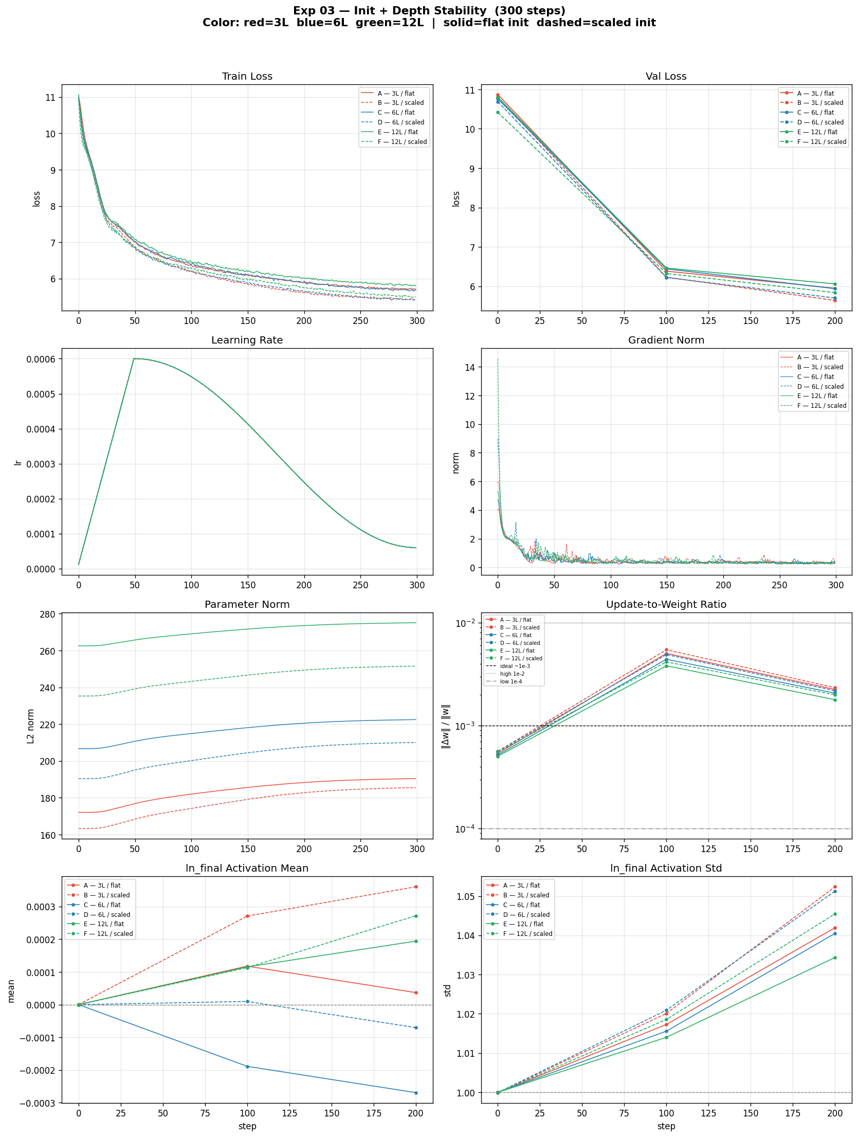
6 variants. Dashed = flat init, solid = scaled. The gap between them grows with depth.
Scaled init converges faster and lower at every depth. The separation is visible from the first few steps and widens throughout. The mechanism is direct: flat init lets each block contribute an uncontrolled amount of variance to the residual stream, so the total variance accumulates proportionally with the number of layers. Gradients flowing backward through this increasingly noisy stream are less coherent, weight updates are less directional, and early training is partially wasted fighting the initialization rather than building useful structure. Scaled init bounds each block’s contribution, keeping the residual stream stable regardless of depth — every gradient step from the start is doing useful work.
The most telling comparison: 12L/scaled ends lower than 3L/flat. A model four times shallower with flat init loses to a full-depth model with clean init. Initialization quality is not a minor hyperparameter at depth — it is a precondition for depth to be useful at all.
Gradient norm shows the same pattern. Early spikes in flat variants are sharper and less coherent, especially at 12L — the same signature as the cold-start problem in Exp 02 (large, incoherent gradients before the optimizer has reliable curvature estimates), but now caused by the initialization rather than the absence of warmup.
The key result is in activation standard deviation. Scaled init produces higher final-layer activation std than flat init at every depth, and the gap widens with depth. This is counterintuitive: scaled init uses smaller initial weights, yet the representations at the final layer are more spread out and discriminative. The explanation is that flat init forces layers to compete — early noisy residual contributions cause later layers to learn defensive near-zero outputs to prevent blowup, so contributions partially cancel across the stream and the network wastes depth. Scaled init lets layers compose — each block adds coherent signal, and the full depth contributes. Higher final activation std is the geometric signature of that: the model is actually using all its layers.
The gap grows with depth. At 3 layers the flat and scaled lines in activation std are close. By 12 layers there is clear separation — larger than the depth effect itself within the flat group. For deeper architectures (24L, 48L) this becomes critical: flat init would produce residual stream variance that layer normalization can no longer reliably suppress.
Takeaway: scaled init is unambiguously better, the benefit compounds with depth, and the mechanism is variance control in the residual stream. All remaining experiments use scaled init as the default.
Exp 04 — Normalization × Learning Rate
What this experiment asks: once init, optimizer, and warmup are settled, the question moves to one of the most consequential architectural choices in transformer design — where layer normalization sits relative to the residual connection. This changes how gradients flow backward through the network, which in turn determines how sensitive the model is to the learning rate.
Layer Normalization (LayerNorm) normalizes the values at each token position to have zero mean and unit variance, then applies learned scale and shift parameters. It prevents any single layer’s activations from growing or shrinking uncontrollably, stabilizing the internal distribution of values throughout the network.
Pre-LN vs Post-LN describes where this normalization sits:
- Pre-LN (used in GPT-2 and most modern transformers): LayerNorm is applied before each sublayer (attention or MLP), inside the residual branch. The residual identity path — the direct bypass from block input to block output — is left un-normalized. The block is:
output = input + Sublayer(LayerNorm(input)). - Post-LN (the original 2017 Transformer paper): LayerNorm is applied after the residual addition, normalizing the combined sum of input and sublayer output together. There is no un-normalized bypass. The block is:
output = LayerNorm(input + Sublayer(input)).
Six variants: Pre-LN and Post-LN each crossed with three learning rates. 1000 steps each, all other settings from the Exp 01 baseline.
| Variant | Norm position | Peak LR | Min LR |
|---|---|---|---|
| A | Pre-LN | 3e-4 | 3e-5 |
| B | Pre-LN | 6e-4 | 6e-5 |
| C | Pre-LN | 1e-3 | 1e-4 |
| D | Post-LN | 3e-4 | 3e-5 |
| E | Post-LN | 6e-4 | 6e-5 |
| F | Post-LN | 1e-3 | 1e-4 |
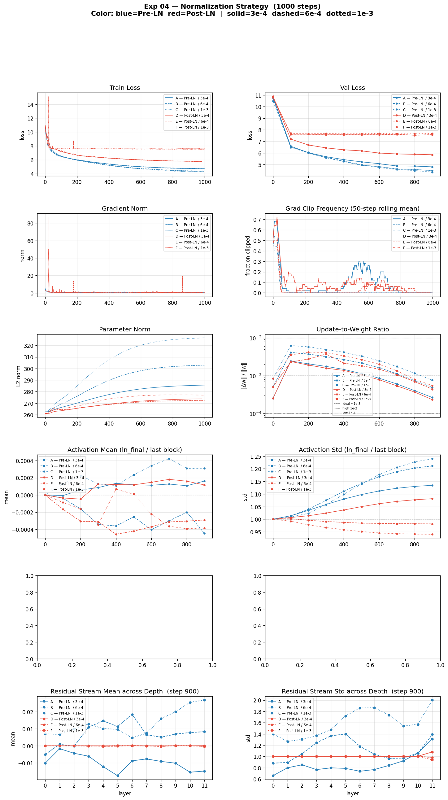
6 variants, Pre-LN solid, Post-LN dashed. The LR sensitivity reversal is the main result.
Pre-LN converged faster and lower at every LR. Best Pre-LN (C, 1e-3) reached a validation loss of 4.35. Best Post-LN (D, 3e-4) reached 5.85 — a gap of ~1.5 nats after 1000 steps. (A nat is simply the unit of the cross-entropy loss when using natural logarithm; lower is better.)
The LR sensitivity reversed between the two variants. In Pre-LN, higher LR produced better final loss: C > B > A. The model was not destabilized at 1e-3 — the gradient path remained clean. In Post-LN the pattern flipped: lower LR produced better final loss. D (3e-4) was the only Post-LN variant that learned meaningfully. E (6e-4) and F (1e-3) essentially stalled after step 100, oscillating near 7.5–7.6 for the remaining 900 steps. That is not slow convergence — it is a training failure.
This reversal is the clearest result in the experiment. LR tolerance is not just a function of model size or dataset — it is directly determined by where normalization sits relative to the residual connection.
The mechanism is in the gradient path. During backpropagation, gradients flow backward through the network to update each layer’s weights. At each block, the gradient splits: one path goes through the sublayer (which includes a LayerNorm), and in Pre-LN, another path goes directly through the identity bypass — un-gated, un-scaled. No matter how LayerNorm transforms the gradient in the sublayer path, the identity bypass delivers the upstream gradient cleanly to the layer below.
In Post-LN there is no such bypass. LayerNorm sits after the residual addition, so every gradient component — including what would have been the identity shortcut — must pass through LayerNorm at every block. LayerNorm is not transparent to gradients: it normalizes activations using the variance of the block’s input, so if that input has high variance (common in early training when weights are random), LayerNorm shrinks the gradient proportionally. Across 12 stacked blocks, this shrinkage compounds. Add a high learning rate on top of that, and the amplified instability causes the training to collapse in the first 100 steps.
Gradient norm was much more erratic in Post-LN throughout training. Early spikes were sharper and more sustained — the direct consequence of LayerNorm gating the full gradient path rather than only the sublayer branch.
Parameter norm was consistently larger in Pre-LN. Post-LN normalizes the residual stream at every block output, which implicitly constrains how large the downstream weights need to grow to handle those activations. In Pre-LN the residual stream accumulates freely across all 12 layers and weights adapt by growing larger. This is not pathological — it reflects that Pre-LN weights are doing more work in absolute terms because the stream is richer.
Residual stream depth profile at step 900 shows the contrast cleanly. Pre-LN: mean near zero across all layers, standard deviation increasing steadily with depth as each block adds structured signal. Post-LN E and F (the failed variants): irregular, oscillating profiles — the network is not building coherent representations across depth.
Takeaway: Pre-LN is unambiguously better across all tested learning rates. The residual identity bypass in Pre-LN allows higher LRs without instability. Post-LN’s lack of bypass makes it LR-sensitive and prone to early training stalls. Pre-LN remains the baseline for all remaining experiments.
What connects them
These four experiments test fundamentally different things — duration, optimizer choice, initialization, normalization placement — but they keep pointing at the same underlying structure: the residual stream is the thing to watch.
Warmup matters because cold optimizer estimates produce step sizes that hammer the residual stream before it has any structure. AdamW without warmup drifts at the final layer because unchecked asymmetry accumulates across 12 residual additions. Flat init’s failure is that it lets each block add uncontrolled variance to the stream, making depth counterproductive. Post-LN’s fragility is that it gates the backward gradient path at every layer, making the entire system sensitive to anything that inflates activation variance — high LR, flat init, no warmup — and any such perturbation compounds across all 12 blocks.
Every signal in the training curves — gradient norm, activation std, parameter norm, residual depth profile — is a different way of observing the same underlying quantity: whether the residual stream is in a regime where each layer can add structured, coherent signal, or whether it is fighting itself.
The practical result of all four: scaled init, AdamW with warmup, Pre-LN, LR around 1e-3 — that is what a stable small transformer pretraining run looks like. Every deviation from that cluster produces a readable signature in the curves.